Predictors of Eviction in Brooklyn, 2010-2016

Overview

Using existing data, we investigated factors that are associated with - and can potentially be used to predict - eviction rates among census tracts in Brooklyn. We used Exploratory Analyses (see navbar menu above) to inform our formal hypotheses and analyses detailed in this section.

We used Generalized Estimating Equations (GEE), which can be used when data are correlated and distinction of within-group and between-group estimates is not desired. Since our data are repeated over time within census tract (2010-2016), we expect there to be autocorrelation present across years, and we can address this using GEE modeling techniques. For more technical information on models used, see the Formal Analysis section of our project report.

Overall, we found that eviction rates are significantly higher, on average, in census tracts with higher proportions of non-white residents (we tested percents of Black, Asian, American Indian / Alaska Native, Native Hawaiian / Pacific Islander, and Hispanic residents). We also found that low-income communities are more at-risk. On average, for every ten percent increase in rent burden (percent of one’s income that is paid for housing), eviction rates are expected to increase 19.29 percent, holding race, year, and population density constant. These results have been shown in previous research and have significant implications for NYC’s affordable housing and eviction landscape.

Analysis

Since our outcome, eviction rate, is calculated using a count variable (number of evictions) repeated over time within areas, we’ll model it using GEE with a Poisson link function.

#####
## poisson distribution of counts (and rates)
joined_data_bklyn_nomissing %>% 
  ggplot(aes(x = eviction_rate)) + 
  geom_histogram(binwidth = 0.1) +
  theme_light() +
  labs(x = "Eviction count per 100 renter-occupied households",
       y = "Count",
       title = "Distribution of eviction counts, standardized by area") +
  theme(plot.title = element_text(hjust = 0.5))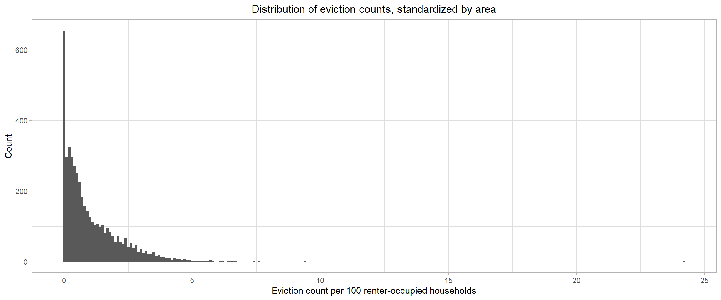

Relevant predictors

Although we formulated specific hypotheses regarding predictors of eviction in Brooklyn based on existing research, we wanted to include as many potential predictors as possible to test against our hypothesized predictors. The data we are using includes the following variables:

evictions. Number of evictions at census level.
eviction_filings. Number of eviction filings at census level.
renter_occupied_households. Number of renter occupied households in census tract. As mentioned above, this forms the denominator of our modelled rate and will be included in all models as an offset term (as log(renter_occupied_households)).
years_since_2010. Since our data range from 2010 to 2016, and we did not want to assume a constant effect of time, we included year as a set of indicator variables in all models except our empty model (see below).
hisp. Percent of population (at census tract level, for all race/ethnicity variables) that self-report Hispanic ethnicity.
white. Percent self-reporting White race.
black. Percent self-reporting Black race.
asian. Percent self-reporting Asian race.
aian. Percent self-reporting American Indian / Alaska Native race.
nhpi. Percent self-reporting Native Hawaiian / Pacific Islander race.
other. Percent self-reporting other race.
rent_burden. Average percent of income spent on rent.
density. Population density.
pct_eng. Percent of population who speak English less than ‘Very Well’. This is interpreted as a proxy for percent English as a second language (ESL) speakers.
median_household_income. Median census tract household income in USD.
poverty_rate. Percent living below Federal Poverty Line (FPL).
median_gross_rent. Median census tract gross rent in USD.
pct_renter_occupied. Percent of census tract occupied by renters.
median_property_value. Median census tract property value in USD.
family_size. Average family size in census tract.
pct_fam_households. Percentage of census tract households that contain families.

Hypothesis

Based on prior reading and research, we hypothesize the following predictors of eviction count at the census tract level. See above for variable definitions.

years_since_2010
rent_burden
density
pct_eng
Race/ethnicity variables (white, black, asian, aian, nhpi, other, hisp)

For detailed model statements, see Report (link in navbar above).

Correlation matrix

Before proceeding, it is important to assess crude correlation among our relevant variables, in case issues of multicollinearity arise during model development.

joined_data_bklyn_nomissing %>% 
  mutate(year = as.numeric(year)) %>% 
  #select(-pct_nonwhite_racedata, -pct_af_am, am_ind_ak_native = aian) %>% 
  select(year, evictions, 
         pct_eng, rent_burden, density, 
         white, black, asian, aian, nhpi, other, hisp,
         median_household_income, poverty_rate, median_gross_rent, median_property_value, pct_renter_occupied,
         family_size, pct_fam_households) %>% 
#  select_if(is.numeric) %>% 
  cor() %>% 
  corrplot::corrplot(type = "lower",
                     method = "square", 
                     addCoef.col = "black", 
                     diag = FALSE, 
                     number.cex = .6,
                     tl.col = "black",
                     tl.cex = .9,
                     tl.srt = 45)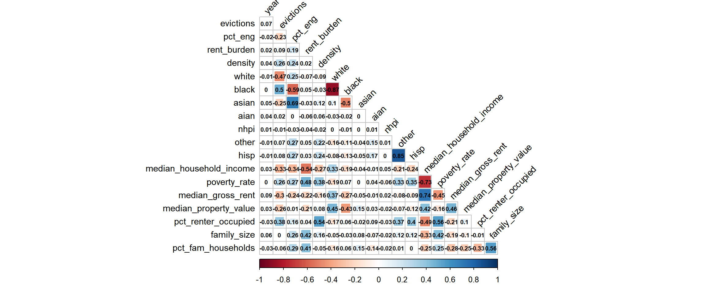

Of relevance to our hypotheses, the following variables were highly correlated and thus may not be accurately interpreted in a model as independent predictors:

pct_eng and year (r = 0.76)
white and black (r = -0.87)
hisp and other race (r = 0.85)

Note on confounding

After performing exploratory data analysis and crude univariate plots (not shown), we found that the relationship between pct_eng - percent of ESL speakers - and eviction rate is confounded by black race.

At first, the relationship between ESL speakers and eviction rate was inverse - as ESL increased, evictions actually decreased. This is counter to our hypotheses, as non-English speaking and immigrant communities have been shown to experience much higher rates of eviction. However, we knew that Black race had the potential to confound this relationship, as Black NYC communities are overwhelmingly English-speaking and also at an increased risk of eviction due to other factors.

Once we adjusted for Black race in the relationship between ESL and evictions, the relationship flipped, and EsL was demonstrated to have a positive association with eviction rate, adjusting for Black race.

Refining and subdefining our hypothesized model

We refined our hypothesized models based on our exploratory confounding and other analyses:

As noted above, ESL should not be included in a model without adjusting for Black race nor should it be interpreted independently of year due to high correlation. Thus, our first hypothesized sub-model will include ESL and percent of all race/ethnicity variables (interpreted as the independent effects of ESL and years since 2010 [highly correlated], rent burden, or population density on evictions, adjusting for each other predictor variable and race/ethnicity).
As also noted above, percent White race and percent Black race are highly correlated in our data (r = 0.87), and percent other race and percent Hispanic ethnicity are also highly correlated (r = 0.85). Thus, a second hypothesized sub-model will observe the independent effects of percent racial/ethnic compositions (excluding White and Other race), rent burden, population density, or years since 2010 on eviction rates, adjusting for other predictor variables.

Stepwise automatic model selection

To contrast with our hypothesis-informed model building process, we wanted to test a stepwise model selection algorithm. We used the gee_stepper function within the pstools package, which performs a forward step selection process with a set of GEE predictors, using QIC to find a ‘best fit’ model.

We slightly modified the function code to create our own function - gee_stepper_o - in order to include our offset term by default in the stepwise selection process.

## use full dataset
full_fit =
  geeglm(evictions ~ 
           offset(log(renter_occupied_households)) + years_since_2010 +
           pct_eng + rent_burden + pct_nonwhite_racedata + density + ## hypothesized
           black + aian + asian + nhpi + other + hisp + ## race
           poverty_rate + pct_renter_occupied + median_gross_rent + median_household_income + median_property_value +
           eviction_filings + family_size + pct_fam_households,
         data = joined_data_bklyn_nomissing,
         id = geoid,
         family = poisson,
         corstr = "ar1")

gee_stepper_o(full_fit, formula(full_fit)) ## customized function to automatically include offset and time covariate

After running stepwise selection, our GEE stepwise model includes predictors:

[offset] - held constant
black
hisp
rent_burden
median_gross_rent
density
poverty_rate
median_household_income
asian
nhpi
aian
pct_renter_occupied

In this model, to be conservative in our interpretations, median_household_income should not be interpreted separately from poverty_rate (r = -0.73) or median_gross_rent (r = -0.74).

Summary of models

To summarize, we will consider the following models to predict census tract-level eviction rates:

Two hypothesized models:

A hypothesized model based primarily on percent ESL speakers [Equation 2, above]
A hypothesized model based primarily on independent effects of race/ethnicity percentages [Equation 3, above]
A model selected via a GEE-specific forward stepwise selection process

In addition to these three models (1, 2, 3), we propose two baseline models:

An empty model, in which there are no predictors, and only the outcome and offset terms are included on opposite sides of the equation, i.e. evictions ~ offset(log(renter_occupied_households))
A naive model, which only uses time to predict eviction rate, i.e. the above model, plus years_since_2010 on the right-hand-side of the model

Cross-validation of models

Since our data are modelled using GEE and are not all nested within each other, there is not a straightforward way to compare their prediction capabilities such as hypothesis testing or AIC (in this case, QIC). However, we can use cross validation, which allows us to compare prediction accuracy across non-nested models. While this technique does not allow us to assess statistical significance of hypotheses/models/predictors tested, we still believe it will be useful in gauging model usefulness.

Specifically, we will compare the repeat-sampled distribution of each model’s root mean squared error, with lower values indicating lower error and better overall prediction.

(For more technical notes, see corresponding section in our report.)

## models
empty_model = ## no predictors
  geeglm(formula = evictions ~ offset(log(renter_occupied_households)),
       data = joined_data_bklyn_nomissing,
       family = poisson,
       id = geoid,
       corstr = "ar1")

naive_model = ## just year
  geeglm(formula = evictions ~ offset(log(renter_occupied_households)) + years_since_2010,
       data = joined_data_bklyn_nomissing,
       family = poisson,
       id = geoid,
       corstr = "ar1")  

hyp_model_eng = 
  geeglm(evictions ~
           offset(log(renter_occupied_households)) +
           years_since_2010 +
           pct_eng + rent_burden + density + 
           white + black + asian + aian + nhpi + other + hisp +
           pct_eng*black,
         data = joined_data_bklyn_nomissing,
         id = geoid,
         family = poisson,
         corstr = "ar1")

hyp_model_race = 
  geeglm(evictions ~
           offset(log(renter_occupied_households)) +
           years_since_2010 +
           rent_burden + density + 
           black + asian + aian + nhpi + hisp,
         data = joined_data_bklyn_nomissing,
         id = geoid,
         family = poisson,
         corstr = "ar1")

step_model = 
  geeglm(evictions ~ 
           offset(log(renter_occupied_households)) + 
           black + hisp + rent_burden + median_gross_rent + 
           density + poverty_rate + median_household_income + asian +
           nhpi + aian + pct_renter_occupied, 
         family = poisson, 
         data = joined_data_bklyn_nomissing, 
         id = geoid, 
         corstr = "ar1")

set.seed(2)

## creating test-training pairs
model_data_cv =
  joined_data_bklyn_nomissing %>%
  crossv_mc(., 100)

## unpacking pairs
model_data_cv =
  model_data_cv %>%
  mutate(
    train = map(train, as_tibble),
    test = map(test, as_tibble))

## assessing prediction accuracy
model_data_cv =
  model_data_cv %>%
  mutate(empty = map(train, ~geeglm(formula = formula(empty_model),
                                      family = poisson,
                                      data = joined_data_bklyn_nomissing,
                                      id = geoid,
                                      corstr = "ar1")),
         naive = map(train, ~geeglm(formula = formula(naive_model),
                                      family = poisson,
                                      data = joined_data_bklyn_nomissing,
                                      id = geoid,
                                      corstr = "ar1")),
         gee_eng = map(train, ~geeglm(formula = formula(hyp_model_eng),
                                      family = poisson,
                                      data = joined_data_bklyn_nomissing,
                                      id = geoid,
                                      corstr = "ar1")),
         gee_race = map(train, ~geeglm(formula = formula(hyp_model_race),
                                      family = poisson,
                                      data = joined_data_bklyn_nomissing,
                                      id = geoid,
                                      corstr = "ar1")),
         gee_step = map(train, ~geeglm(formula = formula(step_model),
                                      family = poisson,
                                      data = joined_data_bklyn_nomissing,
                                      id = geoid,
                                      corstr = "ar1")))

 model_data_cv =
   model_data_cv %>%
   mutate(rmse_empty_gee = map2_dbl(empty, test, ~rmse(model = .x, data = .y)),
          rmse_naive_gee = map2_dbl(naive, test, ~rmse(model = .x, data = .y)),
          rmse_eng_gee = map2_dbl(gee_eng, test, ~rmse(model = .x, data = .y)),
          rmse_race_gee = map2_dbl(gee_race, test, ~rmse(model = .x, data = .y)),
          rmse_step_gee = map2_dbl(gee_step, test, ~rmse(model = .x, data = .y)))

## plotting RMSEs
model_data_cv %>%
  select(starts_with("rmse"), -contains('glm')) %>%
  pivot_longer(
    everything(),
    names_to = "model",
    values_to = "rmse",
    names_prefix = "rmse_") %>%
  mutate(model = fct_reorder(model, rmse, .desc = TRUE),
         model = fct_recode(model, "Empty" = "empty_gee",
                                   "Naive" = "naive_gee",
                                   "Race Model" = "race_gee",
                                   "ESL Model" = "eng_gee",
                                   "Stepwise Model" = "step_gee")) %>%
  ggplot(aes(x = model, y = rmse, fill = model)) + 
  geom_violin() +
  theme_light() +
  labs(x = "Model",
       y = "RMSE", 
       title = "Cross-Validating Models") +
  scale_fill_brewer(type = 'seq', palette = 'Purples') +
  theme(legend.position = 'none',
        plot.title = element_text(hjust = 0.5))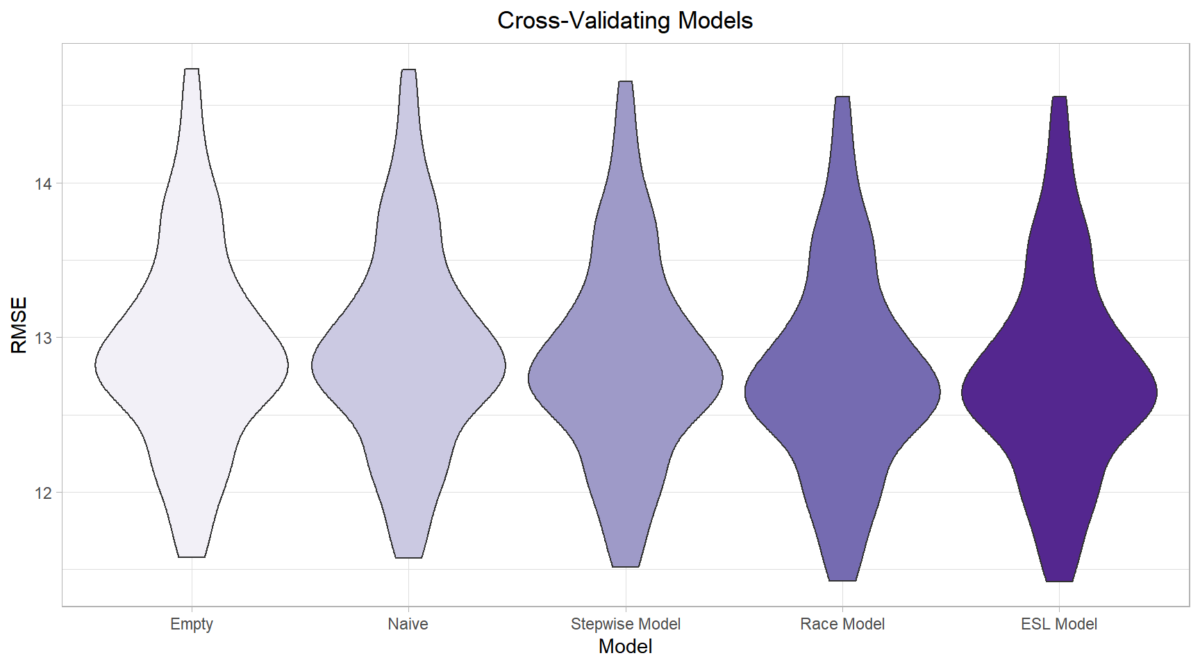

As we can see, our empty and naive models are clearly inferior in terms of their prediction abilities to our other hypothesized and selection-based models.

This is the only clear-cut difference, as the latter three models - our two hypothesized models, and our stepwise model - are very similar in terms of their prediction capabilities.

(Note: None of our models had particularly good predictive capabilities, and the differences between our models given their RMSE distributions is comparatively small. However, we will assume that the difference in RMSE is still meaningful.)

As this is the case, we will opt for model simplicity and select the simplest model with the most easily-interpretable results: the hypothesized model based primarily on the independent effects of non-White race/ethnicity percentages, rent burden, population density, and years since 2010.

Conclusions

Our model can be estimated via GEE:

hyp_model_race = 
  geeglm(evictions ~
           offset(log(renter_occupied_households)) +
           years_since_2010 +
           rent_burden + density + 
           black + asian + aian + nhpi + hisp,
         data = joined_data_bklyn_nomissing,
         id = geoid,
         family = poisson,
         corstr = "ar1")

hyp_model_race %>% 
  broom::tidy() %>% 
  knitr::kable()

term	estimate	std.error	statistic	p.value
(Intercept)	-5.6309476	0.0931704	3652.640062	0.0000000
years_since_20101	-2.9450532	0.0543508	2936.127907	0.0000000
years_since_20102	-0.7230996	0.0244523	874.496766	0.0000000
years_since_20103	-0.8456613	0.0257096	1081.937226	0.0000000
years_since_20104	-0.2351592	0.0220241	114.005530	0.0000000
years_since_20105	-0.3839879	0.0242768	250.180647	0.0000000
years_since_20106	-0.3279125	0.0324796	101.928236	0.0000000
rent_burden	0.0176423	0.0020179	76.439210	0.0000000
density	-0.0000035	0.0000007	24.280014	0.0000008
black	0.0188651	0.0005086	1375.706116	0.0000000
asian	0.0043108	0.0013104	10.822704	0.0010026
aian	-0.0129843	0.0113196	1.315754	0.2513556
nhpi	0.0774339	0.0251317	9.493352	0.0020622
hisp	0.0105379	0.0009028	136.237063	0.0000000

Here, we can see that all hypothesized predictors are significantly associated with eviction rate in Brooklyn except for American Indian / Alaska Native race (p = 0.25) at the 5% level of significance.

Since we used a Poisson (log) link function, we should exponentiate our parameter estimates to get an interpretable estimated measure of effect, interpreted as an estimated risk ratio.

For example, to interpret our parameter estimate for black, we would exponentiate our parameter estimate, 0.01887 (e^0.01887 = 1.0190). This is equal to our estimated risk ratio. We can thus say that the population-average eviction rate (or risk of eviction) is expected to be 1.0190 times higher for each one percentage-point increase in Brooklyn’s Black population, adjusting for percentage of other non-White race/ethnicity (Asian, American Indian / Alaska Native, Native Hawaiian / Pacific Islander, and Hispanic), rent burden, population density, and years since 2010.

To make our risk estimates even more meaningful, we can interpret risk ratios for multiple units. For example, given the above, e^0.01887*10 = 1.2076; for each 10 percent increase in Brooklyn’s Black population, we expect the eviction rate to increase by 21 percent (RRest = 1.21), adjusting for other factors listed in the previous paragraph. Similarly, on average, for every ten percent increase in rent burden, eviction rates are expected to increase 19.29 percent (RRest = 1.1929), adjusting for other factors included in model.

See further discussion in our project report.

Interactive prediction model

We want to enable readers to more easily understand which predictors affect eviction rate and to what extents. Thus, using the race-based GEE model we selected from our five compared models, we created an interactive prediction tool that allows readers to adjust levels of various predictors to see the expected change in eviction rate (evictions per 100 renter-occupied households). Further than the analyses above, readers can also get a sense of these effects in each neighborhood of Brooklyn.

Visit our Prediction Tool to learn more. (You can also find the link in the navbar above.)

Model Building